Forward-Flux

Forward Flux Sampling (FFS) is an enhanced sampling method to simulate “rare events” in non-equilibrium and equilibrium systems. Several review articles in the literature present a comprehensive perspective on the basics, applications, implementations, and recent advances of FFS. Here, we provide a brief general introduction to FFS, and describe the Rosenbluth-like variant of forward flux method. We also explain various options and variables to setup and run an efficient FFS simulation using SSAGES.

Introduction

Rare events are ubiquitous in nature. Important examples include crystal nucleation, earthquake formation, slow chemical reactions, protein conformational changes, switching in biochemical networks, and translocation through pores. The activated/rare process from a stable/metastable region A to a stable/metastable region B is characterized by a long waiting time between events, which is several orders of magnitude longer than the transition process itself. This long waiting time typically arises due to the presence of a large free energy barrier that the system has to overcome to make the transition from one region to another. The outcomes of rare events are generally substantial and thereby it is essential to obtain a molecular-level understanding of the mechanisms and kinetics of these events. “Thermal fluctuations” commonly drives the systems from an initial state to a final state over an energy barrier \(\Delta E\). The transition frequency from state A to state B is proportional to \(e^{\frac{-\Delta E}{k_{B}T}}\), where \(k_{B}T\) is the thermal energy of the system. Accordingly, the time required for an equilibrated system in state A to reach state B grows exponentially (at a constant temperature) as the energy barrier \(\Delta E\) become larger. Eventually none or only a few transitions may occur within the typical timescale of molecular simulations. In FFS method, several intermediate states or so-called interfaces (\(\lambda_{i}\)) are placed along a “reaction coordinate” or an “order parameter” between the initial state A and the final state B (Figure 1). These intermediate states are chosen such that the energy barrier between adjacent interfaces are readily surmountable using typical simulations. Using the stored configurations at an interface, several attempts are made to arrive at the next interface in the forward direction (the order parameter must change monotonically when going from A to B). This incremental progress makes it more probable to observe a full transition path from state A to state B. FFS uses positive flux expression to calculate rate constant. The system dynamics are integrated forward in time and therefore detailed balance is not required.

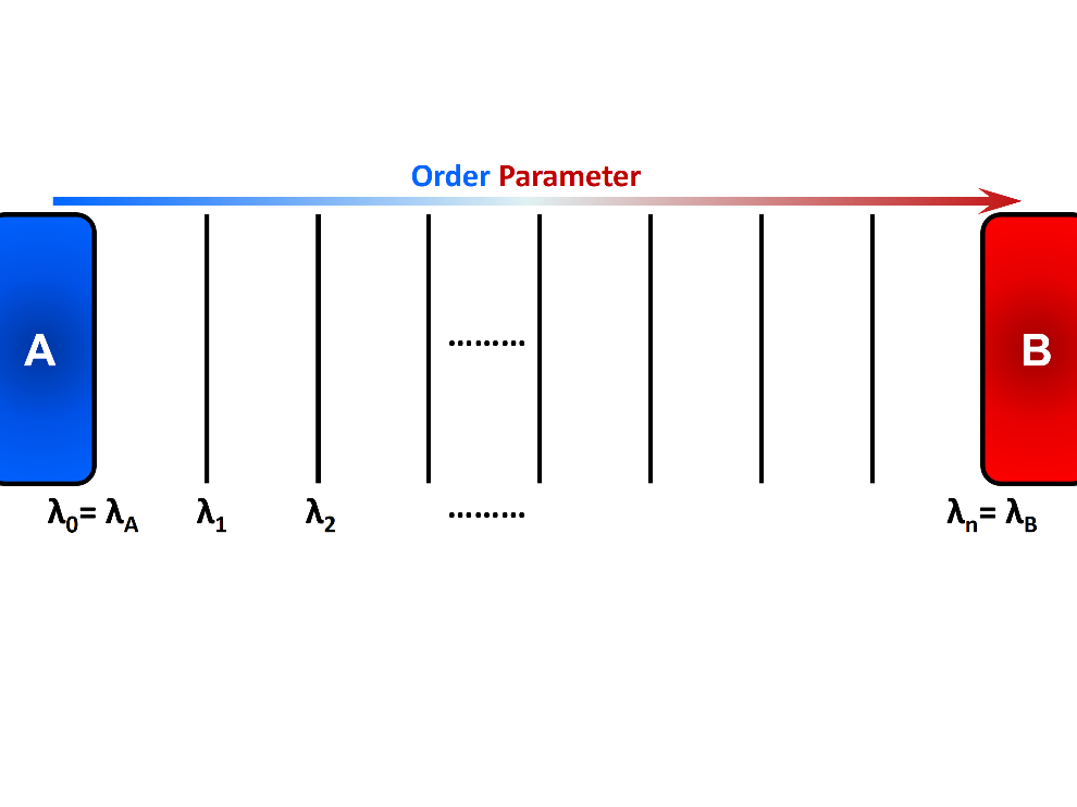
In Forward Flux sampling method, several intermediate states are placed along the order parameter to link the initial state A and the final state B. Incremental progress of the system is recorded and analyzed to obtain relevant kinetic and thermodynamic properties.

Several protocols of forward flux method have been adopted in the literature to

1. generate the intermediate configurations,
2. calculate the conditional probability of reaching state B starting from state A, \(P(\lambda_{B} = \lambda_{n} | \lambda_{A} = \lambda_{0})\),
3. compute various thermodynamic properties, and
4. optimize overall efficiency of the method. The following are the widely-used variants of forward flux sampling method:

• Direct FFS (DFFS) (currently implemented in SSAGES)
• Branched Growth FFS (BGFFS)
• Rosenbluth-like FFS (RBFFS)
• Restricted Branched Growth FFS (RBGFFS)
• FFS Least-Squares Estimation (FFS-LSE)
• FF Umbrella Sampling (FF-US)

Rate Constant and Initial Flux

The overall rate constant or the frequency of going from state A to state B is computed using the following equation:

\[k_{AB} = \Phi_{A,0} \cdot P\left(\lambda_{N} \vert \lambda_{0}\right)\]

here, \(\Phi_{A,0}\) is the initial forward flux or the flux at the initial interface, and \(P\left(\lambda_{N} \vert \lambda_{0}\right)\) is the conditional probability of the trajectories that initiated from A and reached B before returning to A. In practice, \(\Phi_{A,0}\) can be obtained by simulating a single trajectory in State A for a certain amount of time \(t_{A}\), and counting the number of crossings of the initial interface \(\lambda_{0}\). Alternatively, a simulation may be carried out around state A for a period of time until \(N_{0}\) number of accumulated configurations is stored (this has been implemented in SSAGES):

\[\Phi_{A,0} = \frac{N_{0}}{t_{A}}\]

here, \(N_{0}\) is the number of instances in which \(\lambda_{0}\) is crossed in forward direction, and \(t_{A}\) is the simulation time that the system was run around state A. Note that

1. \(\lambda_{0}\) can be crossed in either forward (\(\lambda_{t} < \lambda_{0}\)) or backward (\(\lambda_{t} > \lambda_{0}\)) directions, but only “forward crossing” marks a checkpoint (see Figure 2) and
2. \(t_{A}\) should only include the simulation time around state A and thereby the portion of time spent around state B must be excluded, if any.

In general, the conditional probability is computed using the following expression:

\[P\left(\lambda_{n} \vert \lambda_{0}\right) = \prod\limits_{i=0}^{n-1} P\left(\lambda_{i+1} \vert \lambda_{i}\right) = P\left(\lambda_{1}\vert\lambda_{0}\right)\cdot P\left(\lambda_{2}\vert\lambda_{1}\right) \dots P\left(\lambda_{n}\vert\lambda_{n-1}\right)\]

\(P\left(\lambda_{i+1}\vert\lambda_{i}\right)\) is computed by initiating a large number of trials from the current interface and recording the number of successful trials that reaches the next interface. The successful trials in which the system reaches the next interface are stored and used as checkpoints in the next interface. The failed trajectories that go all the way back to state A are terminated. Different flavors of forward flux method use their unique protocol to select checkpoints to initiate trials at a given interface, compute final probabilities, create transitions paths, and analyze additional statistics.

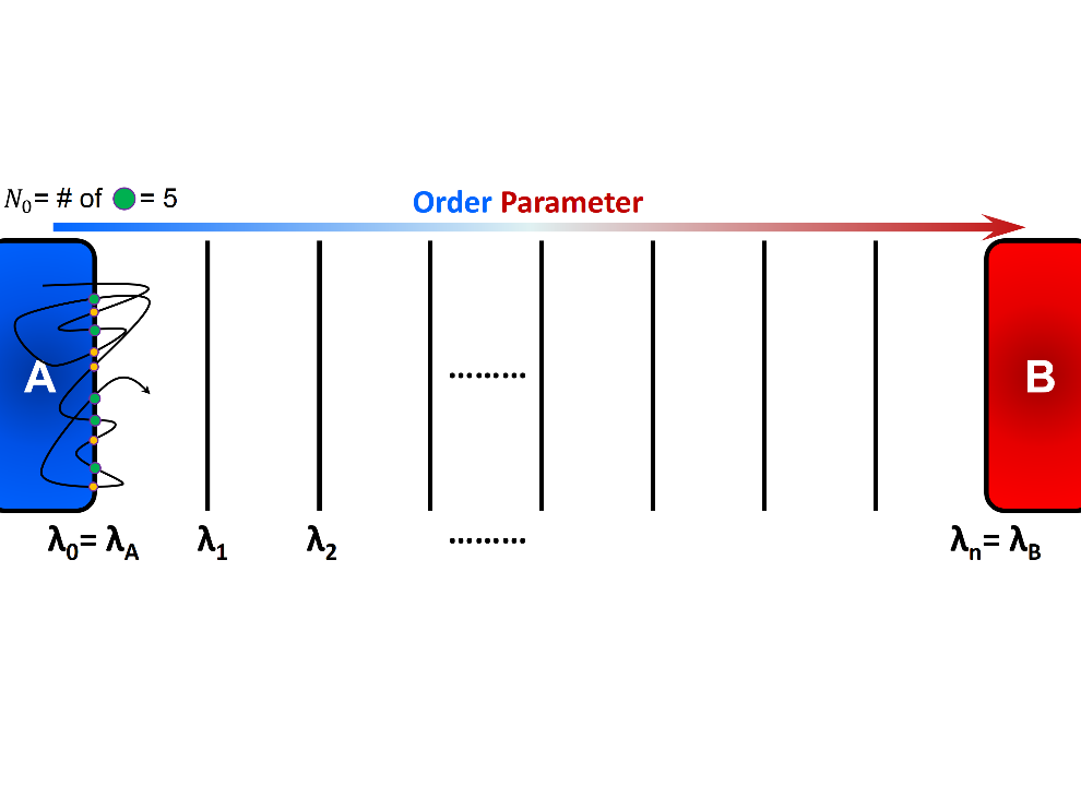
A schematic representation of computation of initial flux using a single trajectory initiated in state A. The simulation runs for a certain period of time \(t_{A}\) and number of forward crossing is recorded. Alternatively, we can specify the number of necessary checkpoints \(N_{0}\) and run a simulation until desired number of checkpoints are collected. In this figure, green circles show the checkpoints that can be used to generate transition paths.

Rosenbluth-like Forward Flux Sampling (RBFFS)

Rosenbluth-like Forward Flux Sampling (RBFFS) method is an adaptation of Rosenbluth method in polymer sampling to simulate rare events [4]. The RBFFS is comparable to Branched Growth Forward Flux (BGFFS) [1] [2] but, in contrast to BGFFS, a single checkpoint is randomly selected at a non-initial interface instead of initiation of trials from all checkpoints at a given interface (Figure 3). In RBFFS, first a checkpoint at \(\lambda_{0}\) is selected and \(k_{0}\) trials are initiated. The successful runs that reach \(\lambda_{1}\) are stored. Next, one of the checkpoints at \(\lambda_{1}\) is randomly chosen (in contrast to Branched Growth where all checkpoints are involved), and \(k_{1}\) trials are initiated to \(\lambda_{2}\). Last, this procedure is continued for the following interfaces until state B is reached or all trials fail. This algorithm is then repeated for the remaining checkpoints at \(\lambda_{0}\) to generate multiple “transition paths”.

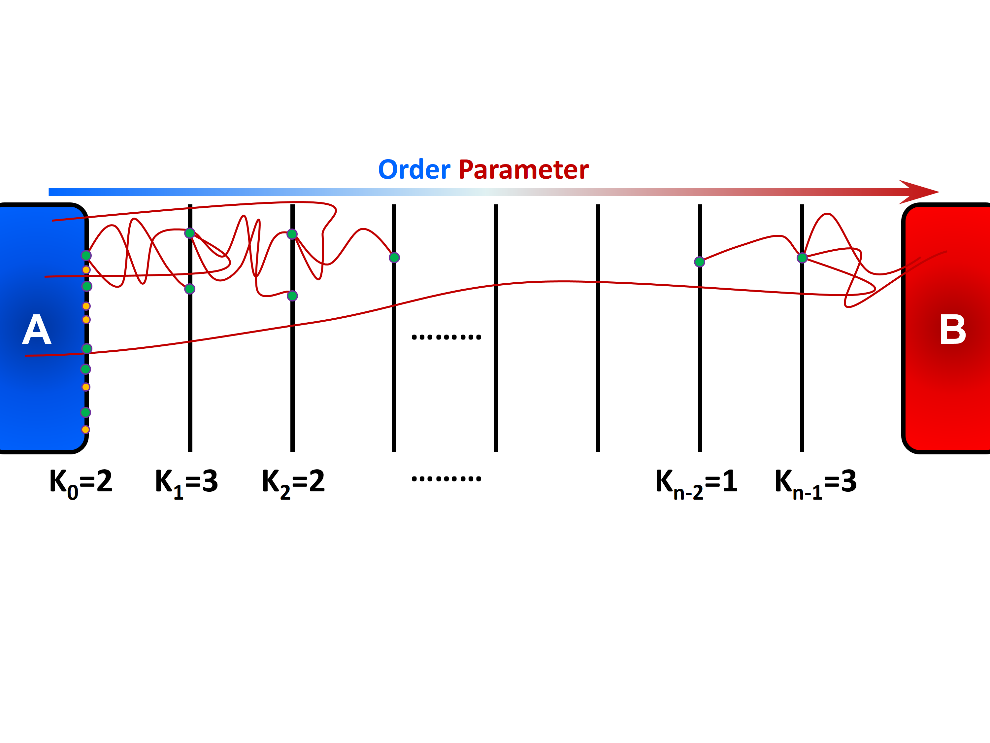
Rosenbluth-like Forward Flux Sampling (RBFFS) involves sequential generation of unbranched transition paths from all available checkpoints at the first interface \(\lambda_{0}\). A single checkpoint at the interface \(\lambda_{i > 0}\) is randomly marked and \(k_{i}\) trials are initiated from that checkpoint which may reach to the next interface \(\lambda_{i+1}\) (successful trials) or may return to state A (failed trial).

In Rosenbluth-like forward flux sampling, we choose one checkpoint from each interface independent of the number of successes. The number of available checkpoints at an interface are not necessarily identical for different transition paths \(p\). This implies that more successful transition paths are artificially more depleted than less successful paths. Therefore, we need to enhance those extra-depleted paths by reweighting them during post-processing. The weight of path \(p\) at the interface \(\lambda_{i}\) is given by:

\[w_{i,b} = \prod\limits_{j=0}^{i-1} \frac{S_{j,p}}{k_{j}}\]

where \(S_{j,p}\) is the number of successes at the interface \(j\) for path \(p\). The conditional probability is then computed using the following expression:

\[P\left(\lambda_{n}\vert\lambda_{0}\right) = \prod\limits_{i=0}^{n-1} P\left(\lambda_{i+1} \vert \lambda_{i}\right) = \frac{ \prod_{i=0}^{n-1}\sum_{p} w_{i,p} S_{i,p} / k_{i} }{ \sum_{p} w_{i,p} }\]

\(\Sigma\) here runs over all transition paths in the simulation.

Options & Parameters

The notation used in SSAGES implementation of the FFS is mainly drawn from Ref. [1]. We recommend referring to this review article if the user is unfamiliar with the terminology. To run a DFFS simulation using SSAGES, an input file in JSON format is required along with a general input file designed for your choice of molecular dynamics engine (MD engine). For your convenience, two files Template_Input.json and FF_Input_Generator.py are provided to assist you in generating the JSON file. Here we describe the parameters and the options that should be set in Template_Input.json file in order to successfully generate an input file and run a DFFS simulation.

Input and parameters related to “walkers”

input

• Type: array of strings
• Default: []
• Functionality: Specifies the name of the engine-specific input files. The user is encouraged to refer to the documentation page of the corresponding MD package to learn about various input options as well as the structure and format of the input files suitable for their MD engine. NOTE: For GROMACS, you won’t need to specify this parameter; instead you’ll need to pass the base name of your .tpr files to “args” (please see the examples folder for details)

logfile

• Type: string
• Default: “log”
• Functionality: Sets the name of the output file that the MD engine uses to write the simulation information including timesteps, energies, etc.

Input and parameters related to “method”

type

• Type: string
• Default: “ForwardFlux”
• Functionality: Instructs SSAGES to activate the “ForwardFlux” module. Do not change this if you plan to run a forward flux sampling simulation.

flavor

• Type: string
• Default: “DirectForwardFlux”
• Functionality: Specifies the flavor of the FFS method that SSAGES should run. Currently, DFFS has been implemented in SSAGES. RBFFS and BGFFS will be available in the future releases.

nInterfaces

• Type: integer
• Default: 5
• Functionality: Sets the total number of interfaces that connects the initial state A to the final State B (including States A and B themselves)

interfaces

• Type: array
• Default: []
• Functionality: Defines an array of intermediate interfaces that links the initial state A to the final state B. This array can either be defined in the Template_Input.json file or FF_Input_Generator.py file. In the latter case, the values of interfaces is left blank in the Template_Input.json file. Minimum of two interfaces must be defined.

N0Target

• Type: integer
• Default: 100
• Functionality: Defines the number of the configurations that ought to be generated (or have been provided by user) at the first interface.

trials

• Type: array
• Default: []
• Functionality: Specifies the number of trials that should be spawned from each interface. The length of this array should match the length of the array of the “interfaces”.

computeInitialFlux

• Type: boolean
• Default: “true”
• Functionality: Specifies whether a calculation of the initial flux should be performed. If this parameter is set to “true”, SSAGES would also generate the user-specified number of initial configurations (N0Target) at the first interface. To compute the initial flux, user must provide an initial configuration in state A, otherwise SSAGES would issue an error. If this parameter is set to “false”, the user must provide the necessary number of the initial configurations in separate files. The files name and the files content should follow a specific format. The format of the files name should be “l0-n<n>.dat” where <n> is the configuration number (i.e. 1, 2, 3, ..., N0Target). The first line of the configuration files includes three numbers “<l> <n> <a>”, where <l> is the interface number (set to zero here), <n> is the configuration number, and <a> is the attempt number (set to zero here). The rest of the lines include the atoms IDs and their corresponding values of positions and velocities, “<atom ID> <x> <y> <z> <vx> <vy> <vz>” where <atom ID> is the ID of an atoms, <x>, <y>, <z> are the coordinates of that atom and <vx>, <vy>, and <vz> are the components of the velocity in the x, y, and z directions. Please note that the stores configurations at other interfaces would follow a similar format.

saveTrajectories

• Type: boolean
• Default: “true”
• Functionality: This flag determines if the FFS trajectories should be saved. Be advised that saving the trajectories of thousands of atoms mandates large storage spaces.

currentInterface

• Type: integer
• Default: 0
• Functionality: Specifies the interface in which the calculations should start from or should continue from. This parameter is helpful in restarting a FFS calculation from interfaces other than State A.

outputDirectoryName

• Type: string
• Default: “FFSoutput”
• Functionality: Specifies the directory name that contains the output of the FFS calculations including the initial flux, the successful and failed configurations, commitor probabilities, and the trajectories. The output data related to the computation of the initial flux is stored in the file “initial_flux_value.dat”, and the data related to transition probabilities is stored in the file “commitor_probabilities.dat”.

Other required input parameters

CVs

• Type: array
• Default: none
• Functionality: Selection of the “order parameter” or the “reaction coordinate”. The current implementation of FFS in SSAGES can takes one collective variable.

Tutorial

This tutorial will walk you step by step through the user example provided with the SSAGES source code that runs the forward flux method on a Langevin particle in a two-dimensional potential energy surface using LAMMPS. This example shows how to prepare a multi-walker simulation (here we use 2 walkers). First, be sure you have compiled SSAGES with LAMMPS. Then, navigate to the SSAGES/Examples/User/ForwardFlux/LAMMPS/Langevin subdirectory. Now, take a moment to observe the in.LAMMPS_FF_Test_1d file to familiarize yourself with the system being simulated.

The next two files of interest are the Template_Input.json input file and the FF_Input_Generator.py script. These files are provided to help you setup sophisticated simulations. Both of these files can be modified in your text editor of choice to customize your input files, but for this tutorial, simply observe them and leave them be. FF_Template.json contains all information necessary to fully specify a walker; FF_Input_Generator.py uses the information in this file and generates a new JSON along with necessary lammps input files. Issue the following command to generate the files:

python FF_Input_Generator.py

You will produce a file called Input-2walkers.json along with “in.LAMMPS_FF_Test_1d-0” and “in.LAMMPS_FF_Test_1d-1”. You can also open these files to verify for yourself that the script did what it was supposed to do. Now, with your JSON input and your SSAGES binary, you have everything you need to perform a simulation. Simply run:

mpiexec -np 2 ./ssages Input-2walkers.json

This should run a quick FFS calculation and generate the necessary output.

Developers

Joshua Lequieu, Hadi Ramezani-Dakhel, Ben Sikora, Vikram Thapar.

References

[1]	(1, 2) R. J. Allen, C. Valeriani, P. R. ten Wolde, Forward Flux Sampling for Rare Event Simulations. J Phys-Condens Mat 2009, 21 (46).

[2]	F. A. Escobedo, E. E. Borrero, J. C. Araque, Transition Path Sampling and Forward Flux Sampling. Applications to Biological Systems. J Phys-Condens Mat 2009, 21 (33).

[3]	R. J. Allen, D. Frenkel, P. R. ten Wolde, Forward Flux Sampling-Type Schemes for Simulating Rare Events: Efficiency Analysis. J. Chem. Phys. 2006, 124 (19).

[4]	M. N. Rosenbluth, A. W. Rosenbluth, Monte-Carlo Calculation of the Average Extension of Molecular Chains. J. Chem. Phys. 1955, 23 (2), 356-359.